PyTorch 입문2

[0] 참고자료

• PyTorch로 시작하는 딥 러닝 입문 유원준 외 1명
• 딥러닝 파이토치 교과서 서지영

[5] 소프트맥스 회귀 Softmax Regression

1. One-Hot Encoding

what?

• 선택해야 하는 개수만큼의 차원을 가지면서, 각 선택지의 인덱스에 해당하는 원소에는 1, 나머지 원소는 0의 값을 가지도락 하는 방법

강아지 = [1, 0, 0]
고양이 = [0, 1, 0]
앵무새 = [0, 0, 1]

why?

예를 들어 강아지 = 1, 고양이 = 2, 앵무새 = 3 라고 레이블을 주었을 때, 손실 함수로 MSE를 사용한다면, 실제 값이 강아지 일 때 예측값이 고양이였다면 (2 - 1)^2 = 1, 실제 값이 강아지 일 때 예측값이 앵무새였다면 (3 - 1)^2 = 4, 즉, 강아지와 고양이가 가깝다는 정보를 주는 결과가 됨

-> 대부분의 분류 문제가 클래스 간의 관계가 균등하므로, 원-핫 인코딩을 많이 사용하게 됨

2. 소프트맥스 회귀

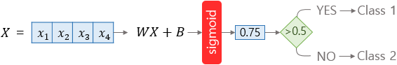
• 로지스틱 회귀

• 소프트맥스 회귀

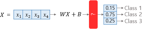
-> 소프트맥스 회귀는 선택지의 개수만큼의 차원을 갖는 벡터를 만들고, 벡터의 모든 합이 1이 되는 어떤 함수를 만들어야 함

• 가중치 계산

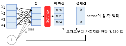
-> One-Hot 인코딩 된 실제값과 비교하여 Weight와 Bias를 업데이트 한다

3. 비용함수 구현하기

1) low-level

import torch
import torch.nn.functional as F

torch.manual_seed(1)

# 3 x 5 크기의 텐서 생성
# 5개의 클래스를 갖는 3개의 샘플
z = torch.rand(3, 5, requires_grad=True)

# 소프트맥스 적용
hypothesis = F.softmax(z, dim=1)

# 임의의 레이블 생성
y = torch.randint(5, (3,)).long()

# 모든 원소가 0의 값을 가진 3 x 5 텐서 생성
y_one_hot = torch.zeros_like(hypothesis)

# y.unsqueeze(1)를 하면 (3,)의 크기였던 y가 (3x1)텐서가 됨 : tensor([[0], [2], [1]])
# scatter 첫번째 인자: dim=1 에 대해 수행
# scatter 세번째 인자: 두번째 인자가 알려주는 위치에 숫자 1
# 연산 뒤에 _가 붙은 경우 덮어쓰기 함
y_one_hot.scatter_(1, y.unsqueeze(1), 1)

# 결과
# tensor([[1., 0., 0., 0., 0.],
#        [0., 0., 1., 0., 0.],
#        [0., 1., 0., 0., 0.]])

# 비용 함수
cost = (y_one_hot * - torch.log(hypothesis)).sum(dim=1).mean()

2) high-level

# 1. low level 수식
#hypothesis = F.softmax(z, dim=1)
#cost = (y_one_hot * - torch.log(hypothesis)).sum(dim=1).mean()
# 2. 축약
cost = (y_one_hot * - torch.log(F.softmax(z, dim=1))).sum(dim=1).mean()

# 3. F.log_softmax
#torch.log(F.softmax(z, dim=1)) 가 많이 사용되므로, F.log_softmax 로 제공됨
cost = (y_one_hot * - F.log_softmax(z, dim=1)).sum(dim=1).mean()

# 4. 잔여 기능이 포함된 함수
cost = F.nll_loss(F.log_softmax(z, dim=1), y)

# 5. 모든 기능이 포함된 함수
cost = F.cross_entropy(z, y)

4. MNIST 데이터 분류

1. MNIST

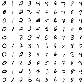
• 숫자 0부터 9까지의 이미지로 구성된 손글씨 데이터셋
• 60,000개의 훈련데이터와 레이블, 10,000개의 테스트 데이터와 레이블로 구성됨
• 레이블은 0부터 9까지 총 10개
• 각 이미지는 28 x 28 픽셀

# torchvision은 유명한 데이터셋들, 이미 구현된 유명 모델들, 일반적인 전처리 도구들을 포함하고 있음
# 자연어처리는 torchtext 사용
import torch
import torchvision.datasets as dsets
import torchvision.transforms as transforms
from torch.utils.data import DataLoader
import torch.nn as nn
import matplotlib.pyplot as plt
import random

# GPU 연산이 가능하다면 GPU 사용
USE_CUDA = torch.cuda.is_available()
device = torch.device("cuda" if USE_CUDA else "cpu")
print("다음 기기로 학습합니다:", device)

# 랜덤시드 고정
random.seed(777)
torch.manual_seed(777)
if device == 'cuda':
    torch.cuda.manual_seed_all(777)

# hyperparameters
training_epochs = 15
batch_size = 100

# MNIST dataset
# root : MNIST를 다운로드 받을 경로
# train : 학습에 사용할지 여부
# transform : 파이토치 텐서로 변환
# download : 데이터가 없을 때 다운로드 받을지 여부
mnist_train = dsets.MNIST(root='MNIST_data/',
                          train=True,
                          transform=transforms.ToTensor(),
                          download=True)

mnist_test = dsets.MNIST(root='MNIST_data/',
                         train=False,
                         transform=transforms.ToTensor(),
                         download=True)

# 데이터 로드
# drop_last : 배치 크기로 데이터를 나누었을 때, 나머지가 발생하면 버릴 지 여부
# 나머지의 갯수가 너무 적은 경우 상대적으로 과대평가 될 수 있음
data_loader = DataLoader(dataset=mnist_train,
                        batch_size=batch_size, # 배치 크기는 100
                        shuffle=True,
                        drop_last=True)

# 모델 설계
# input_dim = 28 x 28 = 784
# output_dim = 10 : 10개의 클래스이므로
# .to() 어떤 장치를 사용해서 연산할 지 지정
linear = nn.Linear(784, 10, bias=True).to(device)

# 비용 함수와 옵티마이저 정의
criterion = nn.CrossEntropyLoss().to(device)
optimizer = torch.optim.SGD(linear.parameters(), lr=0.1)

# torch.nn.functional.cross_entropy()
# torch.nn.CrossEntropyLoss()
# nn 에 포함된 기능은 클래스형, nn.functional에 포함된 기능은 함수형. 기능은 같음

# 학습
for epoch in range(training_epochs): # 앞서 training_epochs의 값은 15로 지정함.
    avg_cost = 0
    total_batch = len(data_loader)

    for X, Y in data_loader:
        # 배치 크기가 100이므로 아래의 연산에서 X는 (100, 784)의 텐서가 된다.
        X = X.view(-1, 28 * 28).to(device)
        # 레이블은 원-핫 인코딩이 된 상태가 아니라 0 ~ 9의 정수.
        Y = Y.to(device)

        optimizer.zero_grad()
        hypothesis = linear(X)
        cost = criterion(hypothesis, Y)
        cost.backward()
        optimizer.step()

        avg_cost += cost / total_batch

    print('Epoch:', '%04d' % (epoch + 1), 'cost =', '{:.9f}'.format(avg_cost))

print('Learning finished')

# 모델 테스트
with torch.no_grad(): # torch.no_grad()를 하면 gradient 계산을 수행하지 않는다.
    X_test = mnist_test.test_data.view(-1, 28 * 28).float().to(device)
    Y_test = mnist_test.test_labels.to(device)

    prediction = linear(X_test)
    correct_prediction = torch.argmax(prediction, 1) == Y_test
    accuracy = correct_prediction.float().mean()
    print('Accuracy:', accuracy.item())

    # MNIST 테스트 데이터에서 무작위로 하나를 뽑아서 예측을 해본다
    r = random.randint(0, len(mnist_test) - 1)
    X_single_data = mnist_test.test_data[r:r + 1].view(-1, 28 * 28).float().to(device)
    Y_single_data = mnist_test.test_labels[r:r + 1].to(device)

    print('Label: ', Y_single_data.item())
    single_prediction = linear(X_single_data)
    print('Prediction: ', torch.argmax(single_prediction, 1).item())

    plt.imshow(mnist_test.test_data[r:r + 1].view(28, 28), cmap='Greys', interpolation='nearest')
    plt.show()

[6] 인공 신경망

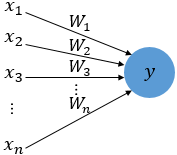
1. 퍼셉트론

1. 퍼셉트론 Perceptron
   • 초기 형태의 인공 신경망
   • 다수의 입력으로부터 하나의 결과를 내보내는 알고리즘

- x :입력 값
- W : Weight 가중치
- y : 출력값

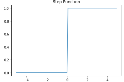
• 각 입력값이 가중치와 곱해져 뉴런에 보내지고, 뉴런에서는 입력값x가중치의 합이 입계치를 넘으면 1을 출력
• 즉, 다음과 같은 계단 함수

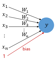
• 임계치를 포함한 퍼셉트론

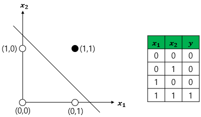
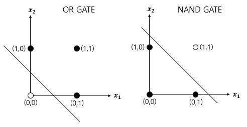
2. 단층 퍼셉트론

• 입력층(input layer), 출력층(output layer) 두 단계로만 구성됨

• 논리게이트 문제

def AND_gate(x1, x2):
    w1=0.5
    w2=0.5
    b=-0.7
    result = x1*w1 + x2*w2 + b
    if result <= 0:
        return 0
    else:
        return 1

def NAND_gate(x1, x2):
    w1=-0.5
    w2=-0.5
    b=0.7
    result = x1*w1 + x2*w2 + b
    if result <= 0:
        return 0
    else:
        return 1

def OR_gate(x1, x2):
    w1=0.6
    w2=0.6
    b=-0.5
    result = x1*w1 + x2*w2 + b
    if result <= 0:
        return 0
    else:
        return 1

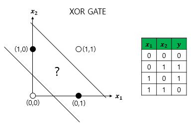
3. 다층 퍼셉트론 MLP MultiLayer Perceptron

• XOR 게이트는 AND, NAND, OR 게이트를 조합하면 만들 수 있음.
• 즉, layer를 더 쌓으면 만들 수 있음

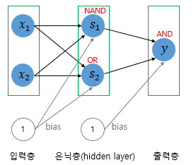
• 이와 같이 입력층과 출력층 사이에 존재하는 것을 은닉층 hidden layer 라 함

import torch
import torch.nn as nn

device = 'cuda' if torch.cuda.is_available() else 'cpu'

# for reproducibility
torch.manual_seed(777)
if device == 'cuda':
    torch.cuda.manual_seed_all(777)

X = torch.FloatTensor([[0, 0], [0, 1], [1, 0], [1, 1]]).to(device)
Y = torch.FloatTensor([[0], [1], [1], [0]]).to(device)

model = nn.Sequential(
          nn.Linear(2, 10, bias=True), # input_layer = 2, hidden_layer1 = 10
          nn.Sigmoid(),
          nn.Linear(10, 10, bias=True), # hidden_layer1 = 10, hidden_layer2 = 10
          nn.Sigmoid(),
          nn.Linear(10, 10, bias=True), # hidden_layer2 = 10, hidden_layer3 = 10
          nn.Sigmoid(),
          nn.Linear(10, 1, bias=True), # hidden_layer3 = 10, output_layer = 1
          nn.Sigmoid()
          ).to(device)

# 비용함수와 옵티마이저 선언
# nn.BCELoss() 는 이진 분류에서 사용하는 크로스엔트로피 함수
criterion = torch.nn.BCELoss().to(device)
optimizer = torch.optim.SGD(model.parameters(), lr=1)  # modified learning rate from 0.1 to 1

# 학습
for epoch in range(10001):
    optimizer.zero_grad()
    # forward 연산
    hypothesis = model(X)

    # 비용 함수
    cost = criterion(hypothesis, Y)
    cost.backward()
    optimizer.step()

    # 100의 배수에 해당되는 에포크마다 비용을 출력
    if epoch % 100 == 0:
        print(epoch, cost.item())

# 학습 결과 확인
with torch.no_grad():
    hypothesis = model(X)
    predicted = (hypothesis > 0.5).float()
    accuracy = (predicted == Y).float().mean()
    print('모델의 출력값(Hypothesis): ', hypothesis.detach().cpu().numpy())
    print('모델의 예측값(Predicted): ', predicted.detach().cpu().numpy())
    print('실제값(Y): ', Y.cpu().numpy())
    print('정확도(Accuracy): ', accuracy.item())