PyTorch 입문

[0] 참고자료

PyTorch로 시작하는 딥 러닝 입문 유원준 외 1명
딥러닝 파이토치 교과서 서지영

[1] 환경 설정(windows)

참고

[2] 기초

1. 데이터 타입

데이터 타입

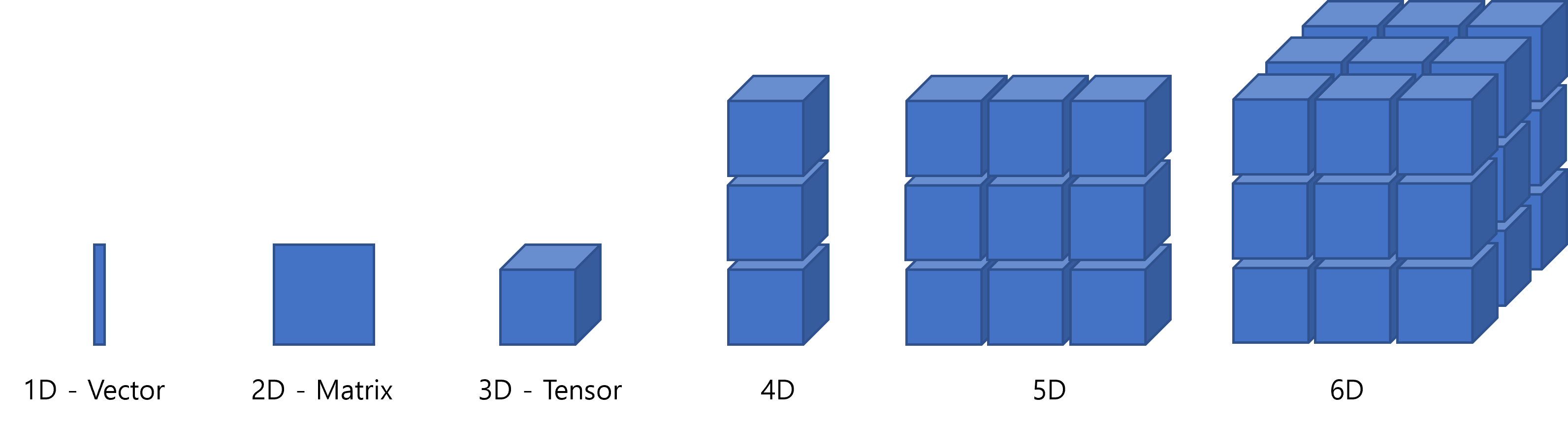
단위 값은 스칼라 Scalar
1차원 배열은 벡터 Vector
2차원은 행렬 Matrix
3차원 텐서 Tensor
상황에 따라 모두가 텐서가 될 수 있음. 1차원 텐서, 2차원 텐서 …

2. 텐서 표기

2.1 2D Tensor |t| = (Batch size, dimension) 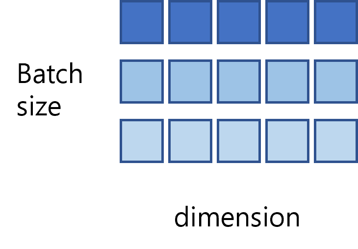데이터 타입

3행 5열 = 3x5
Batch size = 3, dimension = 5

-> 하나의 데이터는 5개의 데이터로 구성되었으며, 한 번에 처리하는 훈련 데이터는 3개이다.

2.2 3D Tensor

|t| = (Batch size, width, height)

하나의 데이터는 width * height로 구성되었으며, 한 번에 처리하는 훈련 데이터는 Batch size만큼이다.

3. 머신러닝 용어

1) 데이터 셋

데이터셋
- 일반적으로 Training, Validation, Testing 세 개의 용도로 분리함
- Validation 데이터는 모덱의 성능을 조정하기 위한 것
- 학습이 종료되면, Validation 데이터에 대해서도 일정부분 최적화가 되었으므로, 성능 테스트에 적합하지 않음
- Training-문제지, Validation-모의고사, Testing-실전시험, 이후 real data 사용
하이퍼파라미터
- 모델의 성능에 영향을 주는 매개변수
- 모델의 성능을 조정하기 위한 용도
- 사용자가 직접 정해줄 수 있는 변수
- ex) learning rate
파라미터
- 학습을 통해 바뀌어져가는 변수

2) Classification & Regression

머신러닝의 많은 문제가 여기에 속함

이진 분류 문제 (Binary Classification)
- 주어진 입력에 대해 둘 중 하나의 답을 정하는 문제
- ex) Pass of Fail, 스팸여부
다중 클래스 분류 (Multi-class Classification)
- 여러 개의 선택지 중 하나의 답을 정하는 문제
- ex) 꽃 품종 분류, 이물질 종류 분류
회귀 문제 (Regression)
- 연속된 값을 결과로 가짐
- ex) 5시간 공부했을 때 80점, 5시간 1분 공부했을 때 80.5점, 7시간 공부했을 때 90점. 그러면 n시간 공부했을 때 점수는?

3) Supervised Learning & Unsupervised Learning

지도 학습
- Label이라는 정답과 함께 학습ㅎ는 것
비지도 학습
- 군집, 차원 축소와 같이 목적 데이터/레이블 없이 학습 하는 방법
강화 학습
- 어떤 환경에서 현재의 상태를 인식하여, 선택 가능한 행동들 중 보상을 최대화 하는 행동 또는 순서를 선택하는 방법

4. Sample & Feature

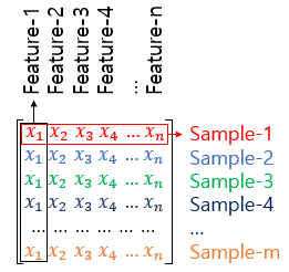
Sample : 하나의 데이터
Feature : y를 예측하기 위한 독립 변수 x

5. Confusion Matrix

정확도 Accuracy
- 맞춘 문제 수 / 전체 문제 수
Confusion Matrix

-	참	거짓
참	TP	FN
거짓	FP	TN

 - True Positive : Positive라 답하고 정답
 - False Positive : Positive라 답하고 오답
 - False Negative : Negative라 답하고 오답
 - True Negative : Negative라 답하고 정답

정밀도 Precision
- 양성이라 답한 케이스에 대한 TP 비율
- precision = TP / (TP + FP)
재현률 Recall
- 양성인 데이터를 실제로 얼마나 양성인지 예측, 즉 재현했는지 비율
- Recall = TP / (TP + FN)
F1-Score
- 정밀도와 재현률은 Trade-off 관계이므로, 적절한 지점을 찾기 위해 조화 평균을 사용함
- 2 * (Precision * Recall / (Precision + Recall))
- TP / (2TP + FN + FP)

6. Overfitting & Underfitting

과적합 Overfitting
- 훈련 데이터를 과하게 학습하여, 훈련데이터에만 적합해진 경우
과소적합 Underfitting
- 훈련을 덜 한 상태

[3] 선형 회귀 Linear Regression

선형 회귀

선형회귀

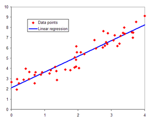
-> x와 y의 선형 관례를 모델링하는 회귀분석 기법

1. Hypothesis

y = Wx + b
H(x) = Wx + b

2. Cost Function

비용 함수(cost function) = 손실 함수(loss function) = 오차 함수(error function) = 목적 함수(objective function)

선형회귀

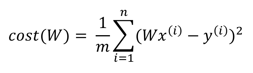
예측 결과와 실제 결과의 차이를 구하는 함수
비용 함수가 최소값이 되게 하는 W와 b를 구하는 것이 목표

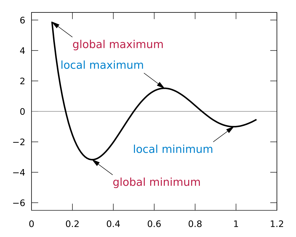
3. Gradient Descent

Cost Function의 값을 최소로 하는 W와 b를 찾을 때 사용하는 것이 Optimizer 알고리즘
Optimizer 알고리즘을 사용해서 W와 b를 찾는 과정을 training
Gradient Descent는 기본적인 Optimizer 알고리즘

경사하강법

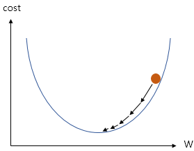
앞서 Cost Function은 W의 값이 너무 커지거나 너무 작아지면 그 결과값이 커진다. (2차원 방정식)
따라서 경사하강법은 cost function의 기울기가 0에 가까운 상태를 찾는다.

2. 구현

  
import torch
import torch.nn as nn
import torch.nn.functional as F
import torch.optim as optim


# 난수 발생 순서와 값을 동일하게 보장해 준다
torch.manual_seed(1)

x_train = torch.FloatTensor([[1], [2], [3]])
y_train = torch.FloatTensor([[2], [4], [6]])

W = torch.zeros(1, requires_grad=True) # size 1,1 인 Tensor 생성
b = torch.zeros(1, requires_grad=True) # requires_grad=True 학습을 통해 변경되는 변수임

optimizer = optim.SGD([W, b], lr=0.01)

nb_epochs = 2000
for epoch in range(nb_epochs + 1):
    # H(x) 계산
    hypothesis = W * x_train + b

    # cost 계산. MSE - Mean Sqaure Error
    cost = torch.mean((hypothesis - y_train) ** 2)

    # cost 계산
    # gradient를 0으로 초기화
    optimizer.zero_grad()
    # 비용 함수를 미분하여 gradient 계산
    cost.backward()
    # W와 b를 업데이트
    optimizer.step()

    # 100번마다 로그 출력
    if epoch % 100 == 0:
        print('Epoch {:4d}/{} W: {:.3f}, b: {:.3f} Cost: {:.6f}'.format(epoch, nb_epochs, W.item(), b.item(), cost.item()))

다중 선형 회귀

  
import torch
import torch.nn as nn
import torch.nn.functional as F
import torch.optim as optim


torch.manual_seed(1)

x_train = torch.FloatTensor([[73, 80, 75],
                             [93, 88, 93],
                             [89, 91, 90],
                             [96, 98, 100],
                             [73, 66, 70]])
y_train = torch.FloatTensor([[152], [185], [180], [196], [142]])

model = nn.Linear(3,1)
print(list(model.parameters()))

optimizer = optim.SGD(model.parameters(), lr=1e-5)

nb_epochs = 2000
for epoch in range(nb_epochs + 1):
    prediction = model(x_train)

    cost = F.mse_loss(prediction, y_train)

    optimizer.zero_grad()
    cost.backward()
    optimizer.step()

    if epoch % 100 == 0:
        print('Epoch {:4d}/{} Cost: {:.6f}'.format(
            epoch, nb_epochs, cost.item()
        ))

new_var = torch.FloatTensor([[73, 80, 75]])
pred_y = model(new_var)
print('result : ', pred_y)

[4] 로지스틱 회귀 Logistic Regression

로지스틱 회귀

둘 중 하나를 결정하는 이진 분류(Binary Classification)을 풀기 위한 대표적인 알고리즘
회귀이지만 분류 작업에 사용함

로지스틱회귀

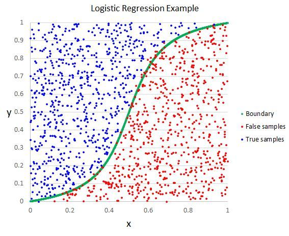
S자 그래프가 그려지므로 새로운 가설이 필요 -> Sigmoid function

시그모이드

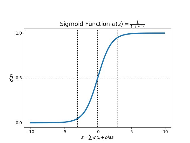
W의 값이 커지면 경사도가 커지고
bias의 값에 따라 그래프가 좌, 우 이동함

구현

  
import torch
import torch.nn as nn
import torch.nn.functional as F
import torch.optim as optim


torch.manual_seed(1)

x_data = [[1, 2], [2, 3], [3, 1], [4, 3], [5, 3], [6, 2]]
y_data = [[0], [0], [0], [1], [1], [1]]
x_train = torch.FloatTensor(x_data)
y_train = torch.FloatTensor(y_data)

model = nn.Sequential(
    nn.Linear(2, 1),
    nn.Sigmoid()
)

optimizer = optim.SGD(model.parameters(), lr=1)

nb_epochs = 1000
for epoch in range(nb_epochs + 1):
    hypothesis = model(x_train)

    cost = F.binary_cross_entropy(hypothesis, y_train)

    optimizer.zero_grad()
    cost.backward()
    optimizer.step()

    if epoch % 20 == 0:
        prediction = hypothesis >= torch.FloatTensor([0.5])
        correct_prediction = prediction.float() == y_train
        accuracy = correct_prediction.sum().item() / len(correct_prediction)

        print('Epoch {:4d}/{} Cost: {:.6f} Accuracy {:2.2f}%'.format(epoch, nb_epochs, cost.item(), accuracy * 100))

print(list(model.parameters()))